In some specific predictive modeling scenarios, we deal with a problem known as "class imbalance." This happens when we want to classify a given example — whether in binary or multi-class tasks — but the training data does not exhibit a balanced distribution of those classes.

Let me use an example to make this clearer. I've been studying some fraud prediction models, specifically frauds known as "Card Not Present Transaction Fraud." These are transactions that occur without the card being physically present, which is very common in online purchases and subscriptions, such as streaming platforms or e-commerce.

With the rise of digital wallets and contactless payments via smartphones or smartwatches, these frauds have become increasingly common. I, for example, almost always leave home without my wallet and rarely use a physical card.

Predicting these frauds is extremely complex, but also very useful for banks, credit card issuers, and payment companies. Beyond the billions of dollars lost to fraud each year, the customer experience can suffer when someone finds a transaction they didn't make, has to cancel their card, request a replacement, file for a refund, and so on. In other words, it's a massive headache — and it typically damages the customer's relationship with the company.

Besides their importance, the fact that these are very rare events makes this task particularly challenging. For every $100 transacted, only 68 cents result from fraud — less than 1%. This means that in a dataset with 100,000 training examples for a classification model, only 680 are fraudulent.

The model then needs to learn to identify fraud from a much smaller number of examples. Without proper precautions, the model can end up specializing in predicting legitimate transactions while struggling — or completely failing — to detect fraud.

This challenge is not unique to financial systems. In other tasks such as churn prediction, cancer cell identification, and resume screening, data scientists face the same challenges.

It's worth noting that, in imbalanced scenarios, binary problems are significantly simpler to work with than multi-class ones. This text is primarily focused on binary cases.

The goal here is to present some of the main techniques for handling class imbalance in classification models. We'll discuss several complementary approaches:

Resampling

There are two main resampling techniques applied before the training step that can help treat imbalanced data: undersampling and oversampling.

Undersampling consists of randomly removing examples from the majority class until the desired distribution or balance between classes is reached. Oversampling follows the same logic, but instead of removing examples, it makes random copies of minority class examples until the desired distribution is achieved.

As you might imagine, both techniques have serious drawbacks that must be considered. When deleting data from your training set, you risk losing relevant data that may hurt the model's generalization, causing underfitting.

The reverse is also true: by duplicating many training examples, the model risks overfitting to those specific training cases.

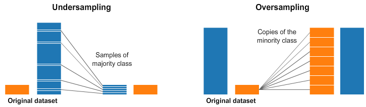
When using resampling techniques, it's important to emphasize that the model should never be tested on the transformed data. Resampling is a technique used during training, and model evaluation must be done on data in its original distribution.

More advanced techniques have been developed to mitigate these fitting risks, while still following the same principle of artificially changing the original distribution of the training set.

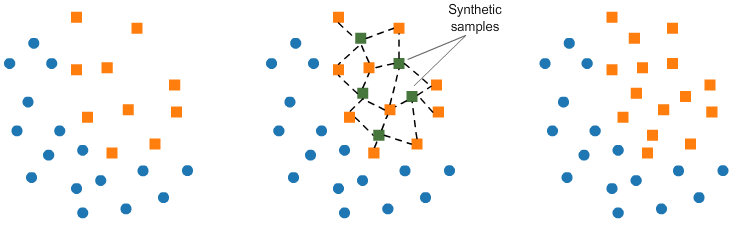
SMOTE (Synthetic Minority Oversampling Technique) is an alternative oversampling method that creates new synthetic examples of the minority class through combinations of existing examples.

This method uses the KNN algorithm to identify and create new samples that follow the same trend as the original data.

Another widely used technique is known as Tomek Links. It identifies pairs of examples from opposite classes that are very close or similar, and then removes them. This creates a clearer separation between the data, making classification easier.

Although this separation helps the model learn more effectively, it can reduce its robustness, since the model loses the ability to handle examples near the decision boundary.

But how do we actually use these techniques? One interesting approach is Two-Phase Learning. In the first phase, a simple initial model (weak learner) is trained on a resampled dataset using techniques like oversampling or undersampling to correct the imbalance. This model captures general patterns in the data, and its predictions can be used as a new feature.

In the second phase, a more robust model is trained on the original data, incorporating this new feature. This process allows the robust model to refine its learning, capture more subtle patterns, and better adapt to minority classes.

This approach not only improves the model's ability to handle imbalance, but also reduces the risk of overfitting to resampled data by using the original dataset in the second phase.

Modeling

Modeling techniques consist of algorithmic-level methods that do not alter the original data distribution but make the model more robust to class imbalance.

This model adjustment can be done through changes to the loss function, which is essentially how many machine learning models learn. In linear models like Linear Regression, the loss function is used to find the line coefficients that minimize the sum of squared errors.

In classification tasks, the most common loss function is called Cross-Entropy. In this function, the weight is the same for all training instances, which means incorrect predictions are penalized regardless of the class.

$$CE(y, \hat{y}) = - \frac{1}{N} \sum_{i=1}^{N} y_i \log(\hat{y}_i) + (1 - y_i) \log(1 - \hat{y}_i)$$

To make our model more robust for fraud detection, we can customize the loss function so that it pays more attention to predicting minority classes. This approach is called "cost-sensitive learning," and there are several functions that can help us achieve this goal. Let's discuss two of them: Class-Balanced Loss and Focal Loss.

The Class-Balanced Loss function makes the weight of predictions inversely proportional to the number of samples from that class in the training set. The core idea is to multiply the original loss term — typically Cross-Entropy — by a weight inversely proportional to the class frequency.

$$W_i = \frac{1}{(1 - \beta) N_i + \beta}$$ $$CB(y, \hat{y}) = \frac{1}{N} \sum_{i=1}^{N} W_i \cdot CE(y_i, \hat{y}_i)$$

During training, this forces the model to pay more attention to instances from underrepresented classes, correcting its natural tendency to favor the majority class. This effect reduces the influence of imbalance on the loss, improving the model's ability to correctly classify examples from underrepresented classes.

The Focal Loss function, on the other hand, is primarily designed to encourage the model to focus on learning from harder examples, assigning greater weight to those predictions. It is a variation of Cross-Entropy that places more weight on hard-to-classify examples and reduces the influence of easy examples.

$$FL(y, \hat{y}) = - \frac{1}{N} \sum_{i=1}^{N} (1 - \hat{P}_i)^\gamma \cdot CE(y_i, \hat{y}_i)$$

During training, the modulation term $(1 - \hat{P}_i)^\gamma$ reduces the impact of already well-classified instances (where the predicted probability $\hat{P}_i$ is close to the correct value), allowing the model to dedicate more effort to instances with higher error.

There are also studies advocating the use of Ensemble algorithms to address class imbalance problems. Although these models weren't originally designed for imbalanced classes and their use is much broader, the structure of Boosting algorithms naturally favors efficiency in these scenarios.

This is because models of this type, such as AdaBoost, have a similar objective to the Focal Loss function. These algorithms use the entire dataset to train classifiers sequentially, focusing on the hardest-to-classify instances. The idea is to correct, at each iteration, the errors made in the previous one.

In this way, they direct greater attention to the most challenging examples using a weight system. Initially, all instances have equal weights. However, after each iteration, the weights of incorrectly classified instances are increased, while those of correctly classified instances are reduced.

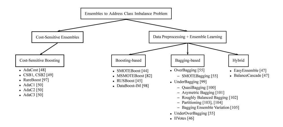
For those wishing to explore the topic further, I recommend reading: A Review on Ensembles for the Class Imbalance Problem: Bagging, Boosting, and Hybrid-Based Approaches

Metrics

In our example, we saw earlier that less than 1% of transactions are considered fraudulent. Often the imbalance between classes is even greater, but let's consider this distribution to simplify some calculations.

Using metrics incorrectly to evaluate these models can lead to accepting poor predictors that haven't learned to correctly detect minority classes, yet appear efficient at first glance.

When using Accuracy (% of correct predictions) as an evaluation metric, for example, a model that simply predicts all transactions as "non-fraudulent" will achieve 99% accuracy without ever correctly identifying a fraud.

This happens because the Accuracy calculation is dominated by the majority class, making it an insufficient metric in cases of severe imbalance.

Moreover, what we want is not to correctly predict legitimate transactions. If that were the case, this "dummy model" would be sufficient. Our goal is to correctly predict the class of interest — in this case, the minority class.

The confusion matrix (or error matrix) is a method for evaluating binary classification models that can help us find more useful metrics. Imagine two models, A and B, trained on the dataset mentioned earlier and used to make predictions on new, unseen data.

Model A	Fraud	Transaction
Prediction: Fraud	2	8
Prediction: Trans.	42	948

Model B	Fraud	Transaction
Prediction: Fraud	9	49
Prediction: Trans.	1	941

Looking at these matrices, which model would you choose? Both models achieved 95% accuracy, but as we've seen, this isn't the most adequate metric for evaluating models in imbalanced class problems. There are more effective metrics such as Precision, Recall, and F1 Score.

Precision evaluates how many cases predicted as fraud were actually fraudulent. Recall, or Sensitivity, corresponds to the percentage of actual frauds that the model managed to capture. In anomaly detection tasks, this is the most important metric.

This means the model is successfully identifying most existing frauds, and few real frauds are being missed. If many real frauds are not being detected by the model, this can be problematic in scenarios where detection is crucial — such as in credit card fraud, where minimizing false negatives is paramount.

Finally, the F1 Score is the combination of Precision and Recall into a single value, functioning as a metric that integrates both to provide a more comprehensive view of model performance.

In some situations, the goal will be to maximize the F1 Score; in others, it may be more important to prioritize Recall, depending on the context and the problem being solved.

Let's see the calculation of these metrics for models A and B:

	Accuracy	Precision	Recall	F1 Score
Model A	0.95	0.02	0.1	0.03
Model B	0.95	0.15	0.9	0.26

Analyzing the evaluation metrics, we can see that despite having the same accuracy, Model B would be the more appropriate choice due to its higher Recall. Remember that this is a simulation designed only to illustrate and help us understand how these metrics work.

For those who want to learn more about how these metrics are calculated, I recommend the article: The Relationship Between Precision-Recall and ROC Curves

Conclusions

Building robust models is inevitably an experimental process that requires continuous adjustments until a satisfactory result is achieved.

From choosing algorithms and evaluation metrics to resampling or adapting the loss function, each approach presents unique challenges and specific benefits that need to be carefully balanced.

I hope I've conveyed that choosing the most appropriate techniques depends on the problem we're trying to solve and the limitations of our data. After all, the goal is always to create a model that not only gets more things right, but gets right what truly matters.

So the next time you encounter a class imbalance problem, remember some of these strategies and techniques to help improve the robustness of your model.

References

[1] C. Huyen, Designing Machine Learning Systems: An Iterative Process for Production-Ready Applications. Sebastopol, CA, USA: O'Reilly Media, 2022.

[2] Nilson Report, "Issue 1187," December 2020. https://nilsonreport.com/newsletters/1187/

[3] M. Galar, A. Fernandez, E. Barrenechea, H. Bustince, and F. Herrera, "A review on ensembles for the class imbalance problem: Bagging, Boosting, and Hybrid-based approaches," IEEE Transactions on Systems, Man, and Cybernetics, Part C (Applications and Reviews), vol. 42, no. 4, pp. 463-484, Jul. 2012. https://doi.org/10.1109/TSMCC.2011.2161285

[4] J. Davis, M. Goadrich. The relationship between Precision-Recall and ROC curves. In Proceedings of the 23rd international conference on Machine learning (ICML '06). Association for Computing Machinery, New York, NY, USA, 233–240, 2006. https://doi.org/10.1145/1143844.1143874

Thanks for reading all the way through! See you next time :)