Machine Learning for Credit Card Fraud Detection

Imagine this: you wake up and head to a bakery for breakfast. When you finish, you go to pay, unlock your phone to tap with a digital wallet—and your purchase is declined.

Later, you decide to take advantage of an end-of-year sale on an e-commerce site. You enter your card details, but the purchase cannot be completed. A message asks you to contact your bank.

You know you have enough money in your account or available credit, yet for some reason the transaction does not go through. One reason may be that more than $30 billion is lost to fraudulent credit card transactions every year. Banks and payment institutions invest heavily in fraud prevention systems.

These systems are not always right. In the situations above, they may have produced false positives. Still, they can prevent significant losses and headaches for both customers and financial institutions.

Card-not-present (CNP) fraud occurs when a purchase is made without the physical card being present. As technology has advanced and online shopping has become more common, these transactions have become widespread.

In Brazil, for example, 61% of consumers prefer shopping online to shopping in physical stores, and 78% make at least one online purchase each month. Customers enter their card number, expiration date, and security code, or use digital wallets on mobile devices. That makes transactions convenient, but also creates more opportunities for fraud.

This article walks through training a classification model to estimate the probability that a transaction is fraudulent and decide whether to approve or reject it. Along the way, we'll discuss class imbalance, dimensionality reduction, and how to choose the right evaluation metrics.

IEEE-CIS Fraud Detection

The data was prepared by the IEEE Computational Intelligence Society and released for the IEEE-CIS Fraud Detection competition on Kaggle.

One particularly interesting aspect is that the data comes from real transactions provided by Vesta Corporation, a company specializing in fraud protection and payment processing for mobile and online transactions. Vesta uses machine-learning models to analyze more than $4 billion in transactions each year, approving purchases in milliseconds and processing payments in over 40 countries.

The dataset contains about 600,000 records and more than 430 features. In addition to the modeling challenge, we need to account for data volume and high dimensionality. Since these are real transactions, most features were anonymized to protect customer privacy, so we do not know what every variable represents.

The Kaggle training data is split across two CSV files. One contains transaction details such as amount, card numbers, location, and product. The other contains identity information, including device type, operating system, internet connection data, and browser version. The tables are joined using TransactionID.

The target variable is isFraud (0 or 1), making this a binary classification problem. Fraudulent transactions (isFraud = 1) account for only 3.5% of the training data, so we are dealing with imbalanced classes.

In an earlier article, I wrote about the challenges of building robust classifiers on imbalanced datasets. I covered techniques such as resampling, class weights, and choosing suitable evaluation metrics. When classes are imbalanced, it is essential to know how to handle the problem effectively.

Accuracy is widely used for general classification problems, but it is not very useful here. Imagine a model that labels every transaction as legitimate. It would be right most of the time and achieve close to 97% accuracy, yet it would be a very poor model.

More useful metrics include precision and recall, which together contribute to the F1 score. They are calculated from true positives, false positives, and false negatives. Depending on the objective, we can tune the model to reduce false positives or false negatives. We'll look at that trade-off in more detail throughout the article.

The Kaggle competition also uses ROC AUC as a benchmark, so I'll use it to compare the model with other solutions built by competitors on the same data. The ROC curve plots the true positive rate (TPR) against the false positive rate (FPR) at different decision thresholds. ROC AUC is the area under this curve and ranges from 0 to 1: 0.5 represents random predictions, and 1 represents a perfect model.

Dimensionality reduction (PCA)

With nearly 600,000 records and more than 400 variables, I used a stratified 10% sample of the original dataset during exploration and experimentation to reduce model training time.

This makes it possible to test different combinations more quickly. Once we've selected a model and its parameters, we can use the full dataset to train the final version. Sampling also allows us to process the data without exceeding available memory.

Stratified sampling creates homogeneous subgroups based on characteristics relevant to the analysis. Here, it is essential to preserve the proportions of fraudulent and legitimate transactions; otherwise, a random sample could make the class imbalance even worse.

I also used a technique to reduce the number of features. A large number of features requires more computing power and can make it harder for a model to generalize.

Principal Component Analysis (PCA) transforms the original features into a new set of uncorrelated variables called principal components. These components are ordered by how much variance they capture, so the first ones explain the largest share. We can discard less informative components, simplifying the model while preserving most of the information.

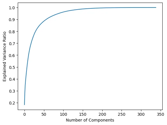
The chart shows cumulative explained variance as the number of principal components increases. It rises quickly at first, which means the initial components capture much of the data's variance. As more components are added, the increase slows because each new component captures a smaller share. Around 50 to 60 components appear to explain a large portion—probably more than 90%—of the total variance.

We can choose an acceptable variance threshold, such as 95%, and determine how many components are needed to reach it. This reduces a high-dimensional dataset to a smaller one, improving algorithm efficiency and reducing the resources needed for training.

Precision vs. recall

One of the most important decisions in credit card fraud detection is finding the right balance between precision and recall. This may be the most important idea in this article.

Imagine a doctor performing routine examinations. For each patient, they must decide whether treatment is warranted based on the symptoms. If they are very cautious and recommend treatment at the slightest sign of illness, few serious cases will be missed (high recall), but many healthy patients will receive unnecessary treatment (low precision).

On the other hand, if the doctor recommends treatment only when absolutely certain, few healthy patients will be treated unnecessarily (high precision), but some serious cases may go unnoticed (low recall).

Fraud detection involves the same dilemma. Precision tells us how many transactions flagged as suspicious really were fraud. Recall tells us how many actual fraudulent transactions we managed to identify. As with the doctor, there is no perfect choice: increasing one usually means reducing the other.

When the model flags a legitimate transaction as fraud (a false positive), the customer is inconvenienced. Their card may be blocked during an important purchase or they may need to answer verification questions. Annoying? Yes. Catastrophic? Not usually.

Now consider the opposite: a real fraud that the model misses (a false negative). The loss can be substantial—not just the money involved, but also the customer's trust in the institution. People are often more understanding of an extra security check than of a failure to protect their money.

This is a constant challenge for financial institutions and should be handled with an understanding of the business. In my view, if we asked bank customers, most would probably prefer not to become victims of fraud, even if that means an occasional transaction is blocked or requires an additional security check.

With this in mind, our goal is a model with strong recall that identifies most fraud without sacrificing too much precision.

That's where the F2 score comes in. Unlike the better-known F1 score, F2 gives more weight to recall. It effectively says: “Precision matters, but missing real fraud matters more.”

The charts below illustrate this trade-off. The first image shows precision and recall moving in opposite directions; it is impossible to maximize both at once. Different models behave differently with respect to these metrics.

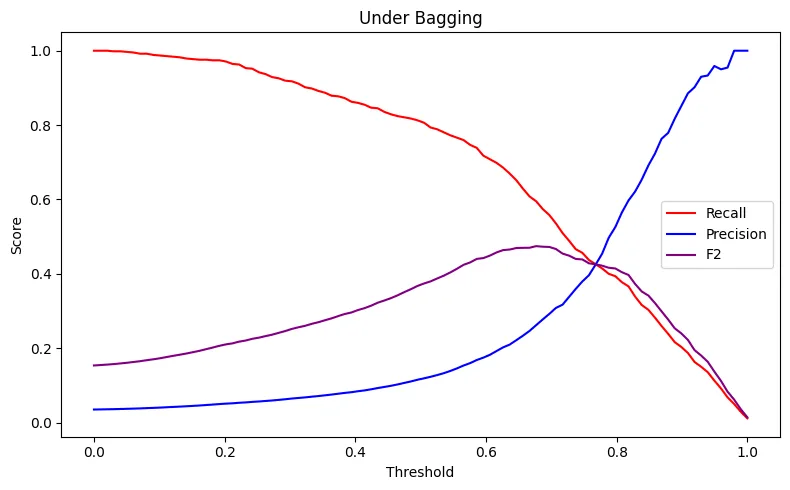
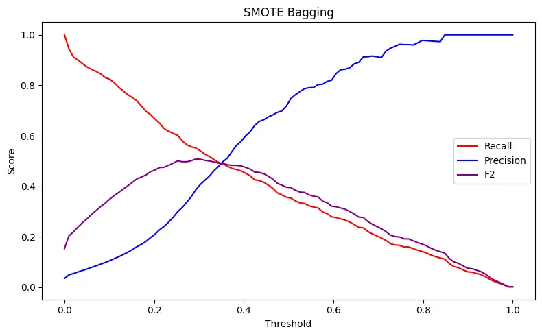
The first chart represents a Random Forest trained on data resampled with RandomUnderSampler(). The second uses SMOTE, which creates synthetic examples of the positive class to help balance the classes.

Both charts show how F2 helps us find a balance that prioritizes the detection of real fraud while still taking precision into account.

In other applications, the trade-off may go the other way. For movie and TV recommendations, as on Netflix, a bad recommendation can frustrate customers and reduce their trust in the service. It may be better not to recommend anything than to recommend something they dislike.

For natural-disaster alerts, false negatives can put lives at risk. In biometric authentication for secure areas, false positives may be more concerning because they could allow unauthorized access.

In fraud detection, we generally lean toward caution: investigate more suspicious cases rather than let real fraud slip through. It is a cost we choose to pay for security.

Model evaluation

Given the model's objectives and its approach to false positives and false negatives, F2 was our primary guide in selecting a model.

I also used ROC AUC as a complementary benchmark, given the Kaggle competition. It helped me determine whether a model was competitive or whether I needed to spend more time on preprocessing and feature engineering.

I tested several model families, especially ensemble methods ranging from LightGBM (boosting) to Random Forests (bagging). Each was tested with different resampling techniques—SMOTE and Random Under-Sampling—to address class imbalance.

When models performed similarly, I chose the one with the higher F2 score, since detecting real fraud was our priority.

The model that came out on top was UnderBagging, combining RandomUnderSampler with Random Forest. It offers a useful mix of performance and efficiency: resampling reduces the number of majority-class examples used for training, speeding up the process.

After selecting the model, I refined the techniques and parameters. First, I simulated possible class-resampling ratios and relative class weights.

Resampling can be complete or partial. Full undersampling makes the classes equal in size, but we can choose a different ratio. The most effective ratio was 1:3, with the minority fraud class representing 33% of the training data.

For class weights, assigning a weight of 2 to fraud and 1 to legitimate transactions produced the best results. In practical terms, the model “pays twice as much” for failing to detect a fraud as it does for a false alarm.

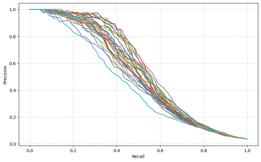
For each simulation, I tracked the chosen metrics (F2 and ROC AUC) and the precision-recall curve. I selected the configurations with the strongest results. The final tuning step used GridSearchCV() to test combinations of hyperparameters for the Random Forest.

Results

After experimentation and refinement, I trained the final model on the complete dataset. The final evaluation used train.py, which contains the full pipeline—from preprocessing and feature creation to training and metric generation. It's worth a look.

	ROC AUC	Precision	Recall	F2 score
UnderBagging	0.91	0.31	0.70	0.56

A ROC AUC of 0.9162 is a particularly good result for fraud detection. Values above 0.9 are generally considered strong because they indicate that the model distinguishes well between legitimate and fraudulent transactions.

The score is competitive: for reference, the winning Kaggle competition model achieved 0.9458, only about three percentage points higher—a small difference given the complexity of the problem.

At first glance, precision of 0.3149 may seem low: only 31% of transactions flagged as suspicious were actually fraudulent. But this reflects our choice to maximize the identification of real fraud. Put another way, for every three transactions flagged, two were legitimate.

The model achieved recall of 0.7055, meaning we caught more than 70% of all fraud. Recall could be pushed closer to 90%, but at too great a cost to precision. The F2 score of 0.5653 reflects this intentional trade-off, giving recall more weight. It represents not just technical performance, but alignment with the business objective.

For reference, training took 20 minutes on a relatively powerful personal computer. That was after resampling, which retained only 11% of the majority class. Without resampling, training would have taken much longer.

Conclusion

I set out to present the main technical challenges in developing a fraud detection model, with particular attention to the trade-off between precision and recall.

Despite the current spotlight on language models and generative AI, traditional machine-learning models remain widely used in industry and perform extremely well on specific problems. Companies such as Stone, Nubank, and Mercado Livre process hundreds of thousands of transactions each day using similar models.

The most critical part of developing these systems is calibrating the model to the specific business context. For fraud detection, that means finding the right balance between false positives and false negatives, accounting for their different costs and the processes used to handle them.

If you'd like to explore the technical details, the complete project code is available on GitHub, including training scripts, experimentation notebooks, and documentation for each step.