Dual Momentum: A Systematic Investment Strategy for Selecting Winning Assets

Momentum strategies are based on the idea that assets with positive returns tend to keep appreciating, while assets with weak or negative returns often continue along the same path.

In other words, momentum is the tendency for asset prices to keep moving in the same direction. Several factors can explain this, including investor behavior: people often follow trends, act irrationally, and get caught up in market narratives.

There are several ways to calculate and apply momentum. Two broad categories are absolute momentum and relative momentum. Absolute momentum looks at an asset's performance against its own price history, asking whether it has delivered positive returns over time.

Relative momentum compares assets to determine which performed best over a given period. Both approaches are widely used to identify assets that may continue to appreciate—or depreciate—based on their past performance.

When academic research in finance was getting started, momentum was not widely accepted. Ideas such as the Efficient Market Hypothesis and the unpredictability of future returns (Random Walk Theory) were dominant.

However, with the growing acceptance of behavioral finance in the early 1970s and the emergence of factors that could help explain asset returns, such as value and size, momentum strategies gained traction.

This study tests a strategy called Dual Momentum, which combines the two approaches: absolute and relative momentum.

Relative momentum is straightforward: compare two assets, and the one with the better performance over the measurement window has greater momentum, or relative strength. Absolute momentum asks whether an asset itself has produced a positive return. One way to measure it is against the risk-free rate. If an asset outperforms the Brazilian CDI rate, for example, we can say it has positive absolute momentum.

The expected outcome of selecting assets based on these signals is a portfolio that generates alpha—excess return at equal or lower risk—relative to benchmarks. The premise of Dual Momentum is to capture risk premiums over the years while occasionally protecting the investor from cycle changes and bear markets by moving into defensive assets.

Applying the model

To test the strategy, I selected the following benchmarks:

• IBOVESPA (Brazilian equities)
• S&P 500 in BRL (US equities converted to Brazilian reais)
• IMA-B 5 (Brazilian government bonds indexed to inflation, with maturities of up to five years)
• CDI (the Brazilian risk-free rate)

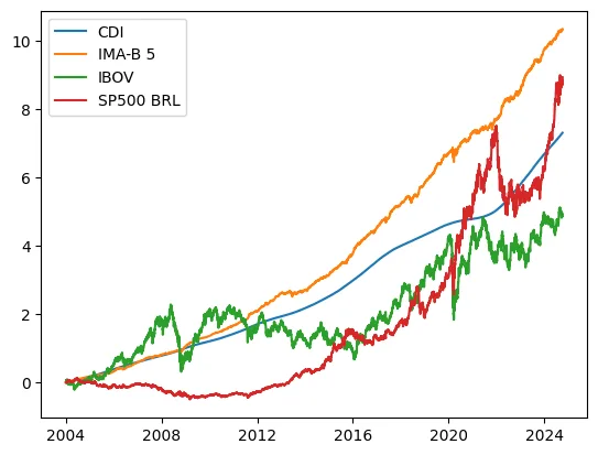
Here's how these benchmarks performed from 2004 onward.

Over a little more than 20 years, IMA-B 5 had the strongest performance. It tracks inflation-linked government bonds (NTN-Bs) with durations of up to five years. It also had relatively low volatility, making it an attractive risk-return balance.

Another notable result is the weak performance of IBOVESPA, whose return was lower than the risk-free CDI rate.

The strategy checks which asset delivered the highest relative return over the past 12 months, invests in it, and rebalances the portfolio monthly. To do this, we need daily closing-price series for the assets and must process them to generate signals and evaluate the strategy. In finance, this process is known as a backtest.

Asset selection worked as follows: first, compare the two risky assets (IBOVESPA and S&P 500) and choose the better performer. Then compare the selected risky asset with the risk-free rate (CDI). If the asset has positive absolute momentum relative to CDI, invest in it. Otherwise, invest in IMA-B 5 until a risky asset outperforms CDI over the 12-month window (Antonacci, 2017).

Backtest

There are two ways to calculate asset momentum: (i) use the return over the last 12 months, or (ii) exclude the most recent month and use the preceding 11 months within that 12-month window.

The last month is sometimes excluded because research, including Jegadeesh and Titman (1993), finds that momentum strategies that leave it out tend to outperform those using all 12 months. The idea is to capture a sustained trend while avoiding the effect of short-term reversals.

Behavioral-finance research has found that, in the short term, asset returns can be influenced by reversal movements, particularly during the most recent month. For that reason, this backtest excludes the latest month when calculating the 12-month return.

I calculated returns on the first trading day of each month. This makes it possible to rebalance monthly, evaluate each asset's momentum, and decide where to invest.

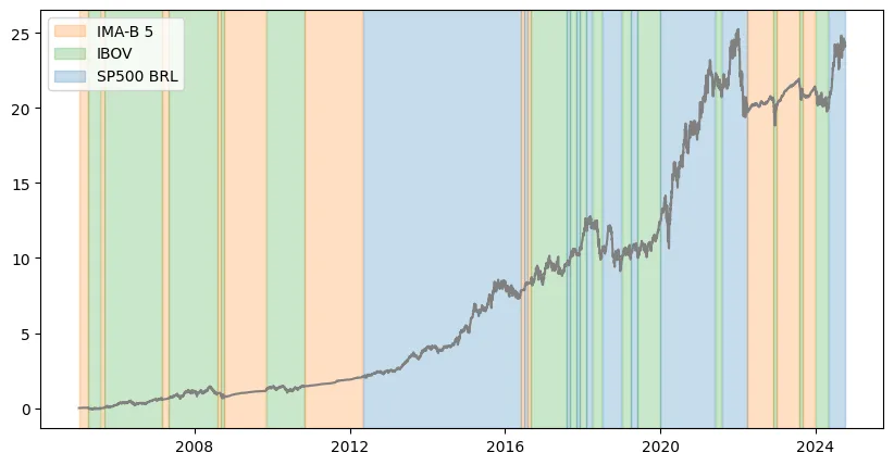
Under this strategy, the portfolio spent approximately 40% of the time invested in the S&P 500, 35% in IBOVESPA, and 25% in IMA-B 5.

The chart shows the periods in which the model held each asset, as well as the momentum shifts—points where the trend changed.

Benchmark and model evaluation

A useful way to assess an investment strategy or model is to compare it with a benchmark. Beyond checking whether it outperformed each asset individually, we can compare it with a simple reference portfolio.

I created a naive portfolio that invests equally in the three assets. An investor could build this equal-weight portfolio and rebalance it monthly without much effort. A more sophisticated strategy should aim to outperform this baseline.

	CAGR	Volatility	Sharpe ratio
IBOV	8.92%	26.58%	-0.0404
CDI	10.44%	0.23%	1.8691
Naive Portfolio	11.28%	12.37%	0.1035
IMA-B 5	12.13%	2.85%	0.7477
S&P 500 BRL	12.14%	20.89%	0.1024
Dual Momentum	17.72%	19.64%	0.3931

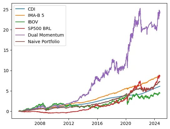
Looking at the risk (volatility) and return (CAGR) metrics, the strategy comfortably outperformed the equal-weight portfolio, returning more than 17% a year over the past 20 years, though with higher volatility.

Despite the higher volatility, its Sharpe ratio—return per unit of risk—was also higher, suggesting a better risk-return relationship.

I kept CDI in the comparison because it is the risk-free rate used to calculate momentum. However, the model behaved more like a risky asset than a defensive one, given its volatility. So let's also compare it with the other risky assets, the S&P 500 and IBOVESPA.

Although Dual Momentum was volatile, like other risky assets, it delivered a higher return than the other assets analyzed. Its volatility was similar to that of the S&P 500, but it produced approximately 5.5 percentage points of excess return per year.

The strategy's volatility is partly characterized by a phenomenon known as momentum crashes: abrupt, severe reversals in assets that had been performing well. Notable examples occurred in 2008 and 2020. In 2020, the COVID-19 pandemic triggered significant declines in global risk assets.

Researchers have studied these events extensively and continue to develop methods to mitigate their effects, including more advanced volatility and trend-reversal forecasts.

Drawdowns

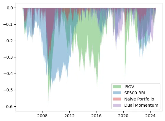
Since the strategy behaved more like a risky asset, it is useful to analyze its drawdowns, or declines from previous peaks. Understanding the strategy's risk also means looking at the magnitude and duration of drawdowns, which gives us a clearer picture of recovery periods and their impact on overall performance.

	Average duration	Maximum duration	Largest drawdown
Naive Portfolio	8 days	377 days	-36%
Dual Momentum	11 days	691 days	-33%
S&P 500 BRL	20 days	2,017 days	-52%
IBOV	23 days	2,304 days	-60%

Despite the risk of momentum crashes, the strategy had shallower and shorter drawdowns than the other risky assets. This suggests that even during corrections, it recovered more quickly and reduced the severity of losses compared with traditional risk assets.

Maximum drawdown duration matters. An investor unlucky enough to buy IBOV at the wrong point during this period could have spent more than six years underwater before recovering their investment.

That doesn't even account for opportunity cost: during that time, the investor could have held CDI, with no market risk. In other words, the loss was substantial.

Rolling 10-year windows

Another way to evaluate the strategy while reducing the bias of choosing a particular time window is to test every possible 10-year period since 2004. We have seen that the model outperformed all the benchmark assets over the last 20 years, but does that hold for other windows as well?

I went back to the code, calculated daily index returns, identified every possible 10-year window, and ran the backtest again for each one.

Across more than 2,600 windows, the strategy outperformed CDI in 100% of them and delivered an average return equal to 337% of CDI.

Conclusion

Dual Momentum proved effective for the goals of this study, delivering strong returns (+17% a year) over the past 20 years with lower volatility than other risky assets such as the S&P 500 and IBOVESPA.

Still, despite its strong returns, the strategy has some drawbacks.

It is simple, but it requires considerable discipline, especially during periods of high volatility. Although it can help investors avoid long bear markets, there is a risk of tracking error: over shorter periods, the strategy may underperform risky assets.

As the backtest showed, the strategy is also exposed to momentum crashes, which can make it quite volatile at times and cause losses if an investor lacks discipline or abandons the strategy.

These issues are common to other momentum strategies. One positive feature of this particular approach is that investors can replicate it easily and transaction costs are relatively low, since it involves few assets and infrequent trades.

An investor who had followed the strategy since 2004 would have made fewer than two trades a year on average over the following 20 years. That means simple portfolio management and low operating costs.

In Brazil, investors can replicate the strategy using ETFs (exchange-traded funds), which track indexes or specific assets and offer a practical combination of diversification and liquidity. The relevant ETFs are:

• BOVA11 (IBOVESPA)
• IVVB11 (S&P 500)
• B5P211 (IMA-B 5)

For a more accurate return analysis, we would need to account for the ETFs' management fees. Although relatively low compared with the rest of the fund industry, they still affect final returns. Trading costs should also be included. I did not account for them in this study, so they are an important consideration for future work and for estimating net returns more realistically.

References

[1] Antonacci, Gary, “Risk Premia Harvesting Through Dual Momentum” (October 1, 2016). Journal of Management & Entrepreneurship, vol. 2, no. 1 (March 2017), 27–55. SSRN or DOI.

[2] Jegadeesh, N. and Titman, S. (1993), “Returns to Buying Winners and Selling Losers: Implications for Stock Market Efficiency.” The Journal of Finance, 48: 65–91. https://doi.org/10.1111/j.1540-6261.1993.tb04702.x