An End-to-End Data Pipeline Using Brazil's ANS Data with Databricks, AWS, and Spark

Objective

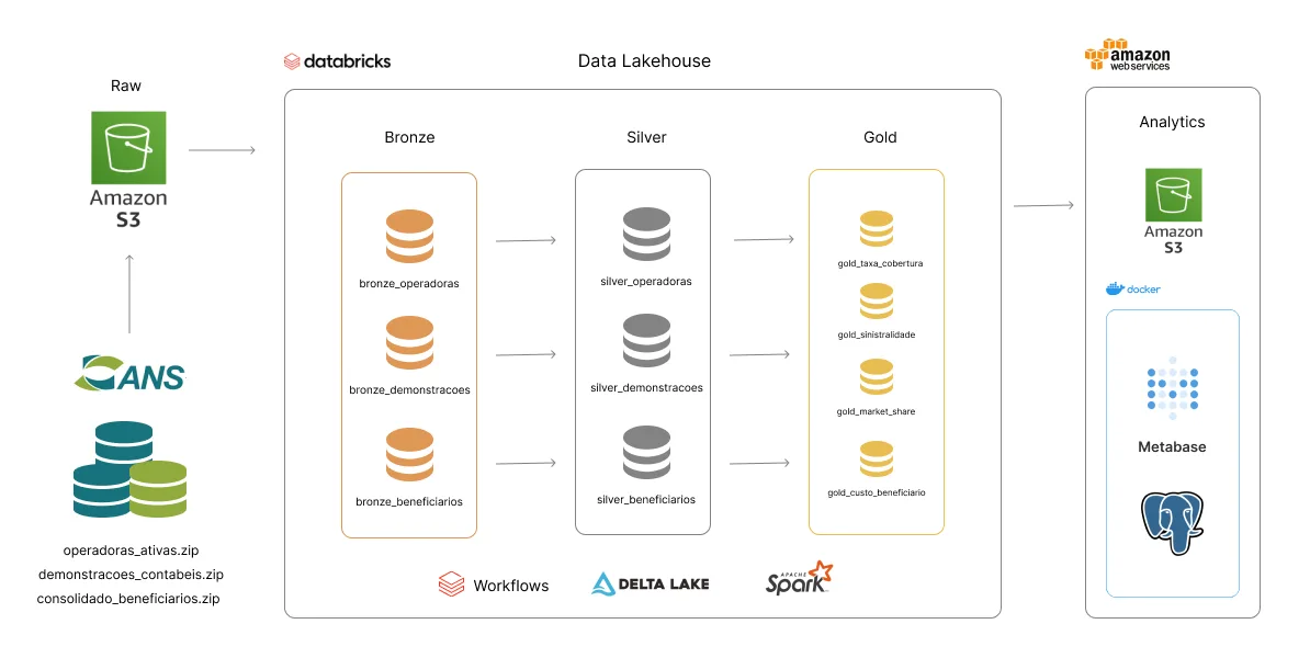
The goal of this project was to build an end-to-end data pipeline covering ingestion, modeling, transformation, and loading, using Databricks on AWS. At the end, I also analyzed the data to answer a set of questions.

The data comes from Brazil's Agência Nacional de Saúde Suplementar (ANS), the National Supplementary Health Agency, which publishes large open datasets about health-insurance providers and their members.

Some datasets contain tens or even hundreds of gigabytes, making them a useful way to put distributed processing, data lakehouse modeling, and Apache Spark architecture into practice.

I used a Databricks Premium free trial and AWS as the cloud environment for the workspace. I was already familiar with AWS, but Azure and GCP could also be used. I chose not to use Databricks Community because I wanted hands-on experience with an environment closer to those used by companies, including essential features such as Databricks Workflows for orchestration and GitHub repository integration.

The Premium version incurred costs, which I'll discuss later. I also used EC2 instances in addition to the Databricks clusters for the analytics portion of the project.

Questions

The analyses were designed to answer the following questions:

1. What is the current medical loss ratio in the health-insurance sector?
2. Which insurer is most efficient in terms of cost per member?
3. What is each insurer's market share by number of members in the medical and hospital segment?
4. How many health-plan companies operate in Brazil?
5. How many people in Brazil have health-insurance coverage? What is the coverage rate?
6. Are individual or group plans more common?

Data collection

ANS publishes its open data through an FTP server, available at dadosabertos.ans.gov.br/FTP/PDA.

Overall, the data is well organized and of good quality. Most datasets include metadata or a catalog; some catalogs even identify columns that are foreign keys to other datasets, which is especially helpful.

Some of the datasets are very large. The monthly active-beneficiary registry, for example, contains around 10 GB of CSV files, totaling approximately 14.5 million records and 22 attributes for each month.

The files are distributed as ZIP archives. The collection code extracts them, reads them into memory, and persists them to a Databricks volume (or S3 storage), which acts as the raw landing layer.

Persisting the source files in raw storage outside Delta Lake helps avoid common problems when handling large datasets and Spark clusters, such as spill.

After saving the files to storage, I read them with pyspark and ingested them into the bronze layer in Delta format. Bronze ingestion was implemented with ingestion classes, such as bronze_beneficiarios.py.

Data modeling

For this project, I chose to create a data lake: a place to store structured and unstructured data in its original form, without imposing a schema up front, for downstream processing or applications.

The challenge with traditional data lakes is that data is saved as collected, often with low quality and without constraints or processing layers.

One widely used solution, especially among Databricks users because of its easy integration, is the open-source Delta Lake framework and the lakehouse architecture.

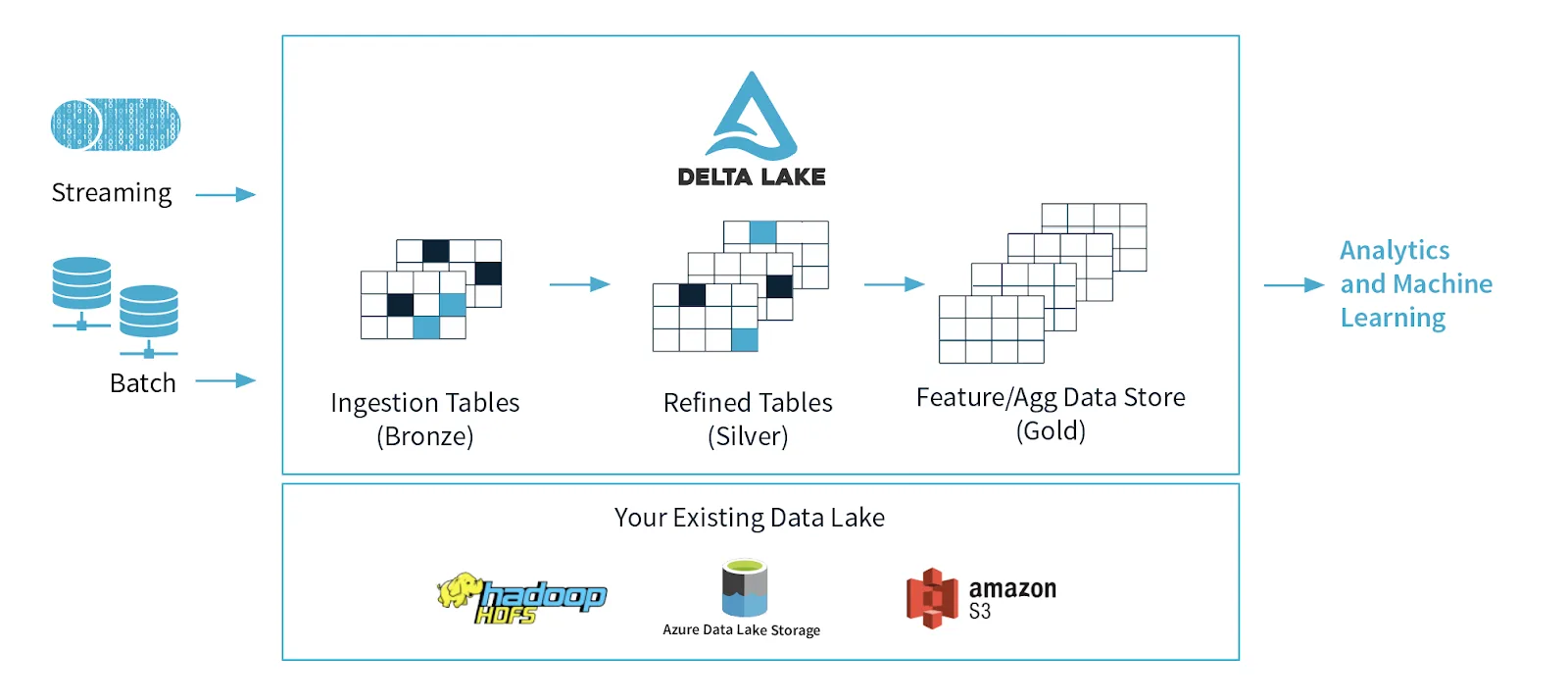
Delta Lake is an abstraction layer built on top of a traditional data lake such as Amazon S3. It encourages layered data flows in which data is progressively cleaned and improved. The layers are:

• Bronze: raw tables that preserve the collected data as faithfully as possible.
• Silver: tables with defined schemas, cleaned and enriched data.
• Gold: aggregated tables built around business rules and metrics of interest.

Data lineage and metastore

Saving tables in Delta format and using Unity Catalog provides access to integrated Databricks metastore features, including access control, usage metrics, schema views, and data lineage.

The lineage diagram below shows gold.ans.custo_beneficiario, a table built from four source tables:

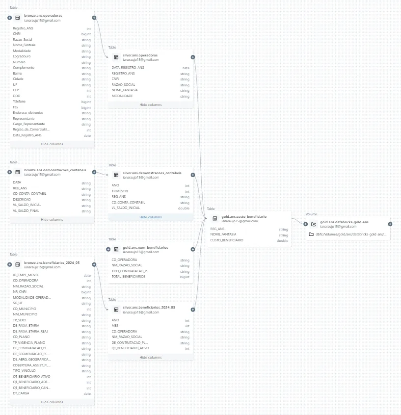
The bronze-layer schemas (on the left of the image) have more dimensions and include data with unsuitable types, inconsistent column names, and other signs of lower-quality source data.

One example is the CNPJ column in bronze.ans.operadoras. Spark inferred it as a bigint, even though it should be a string. That change is made in the silver layer, where silver.ans.operadoras uses the correct type.

The transformation code is available in silver_operadoras.py:

df = spark.sql(f'SELECT * FROM bronze.{schema}.{table}')

upper_cols = [col.upper() for col in df.columns]
df = df.toDF(*upper_cols)

final = df \
    .withColumn('REGISTRO_ANS', df['REGISTRO_ANS'].cast('string')) \
    .withColumn('RAZAO_SOCIAL', F.regexp_replace(F.col('RAZAO_SOCIAL'), r'[./]', '')) \
    .withColumn('RAZAO_SOCIAL', F.regexp_replace(F.col('RAZAO_SOCIAL'), r'\\b(LTDA|SA|EIRELI|ME|EPP)\\b', '')) \
    .withColumn('RAZAO_SOCIAL', F.regexp_replace(F.col('RAZAO_SOCIAL'), r' - $', '')) \
    .withColumn('CNPJ', df['CNPJ'].cast('string')) \
    .select(
        'DATA_REGISTRO_ANS',
        'REGISTRO_ANS',
        'CNPJ',
        'RAZAO_SOCIAL',
        'NOME_FANTASIA',
        'MODALIDADE'
    )

final = final.withColumn('NOME_FANTASIA', F.when(
    F.col('NOME_FANTASIA').isNull(), F.col('RAZAO_SOCIAL')).otherwise(F.col('NOME_FANTASIA')
))

final.write.mode('overwrite').format('delta').saveAsTable(f'silver.{schema}.{table}')

The code casts CNPJ to a string. It also cleans RAZAO_SOCIAL, removing common company suffixes such as LTDA, SA, EIRELI, and ME. When NOME_FANTASIA is NULL, it uses RAZAO_SOCIAL instead.

Example: cost per member

As tables move through the pipeline, their schemas become more defined. The final gold tables are consumed by the analytics environment to generate insights and data products such as dashboards.

gold.ans.custo_beneficiario is a useful example. It calculates an indicator of insurer efficiency by combining all three primary data sources.

I used SQL for most transformations in the gold layer:

CREATE OR REPLACE TABLE gold.ans.custo_beneficiario
USING DELTA AS (
  WITH despesas AS (
    SELECT ANO, REG_ANS, AVG(VL_SALDO_INICIAL) AS TOTAL_DESPESAS
    FROM silver.ans.demonstracoes_contabeis
    WHERE ANO = 2023 AND CD_CONTA_CONTABIL = '41'
    GROUP BY ANO, REG_ANS
  ),

  beneficiarios AS (
    SELECT CD_OPERADORA, SUM(TOTAL_BENEFICIARIOS) AS NUM_BENEFICIARIOS
    FROM gold.ans.num_beneficiarios
    GROUP BY CD_OPERADORA
  ),

  operadoras AS (
    SELECT * FROM silver.ans.operadoras
    WHERE LOWER(MODALIDADE) NOT LIKE '%odonto%'
  )

  SELECT d.REG_ANS, o.NOME_FANTASIA, ROUND(d.TOTAL_DESPESAS / b.NUM_BENEFICIARIOS, 2) AS CUSTO_BENEFICIARIO
  FROM despesas AS d
  LEFT JOIN beneficiarios AS b ON d.REG_ANS = b.CD_OPERADORA
  LEFT JOIN operadoras AS o ON d.REG_ANS = o.REGISTRO_ANS
  WHERE b.NUM_BENEFICIARIOS > 0 AND d.TOTAL_DESPESAS > 0
);

The final gold table has only three fields:

Field	Type	Description
REG_ANS	string	ANS insurer identification code
NOME_FANTASIA	string	Insurer's trade name
CUSTO_BENEFICIARIO	double	Quarterly cost per member, in Brazilian reais (R$)

This table can feed dashboards or be joined with other tables, such as gold.ans.market_share, to compare efficiency among market leaders.

Loading and orchestration

All ETL stages—extraction, transformation, and loading—were automated using Python (pyspark), SQL, and Databricks Workflows.

If we include ingestion into the raw layer, the process is more accurately described as ELT (extract, load, transform): source CSV files are collected and loaded into a landing zone in their original format, then transformed into Delta tables.

I chose this approach because of the large volume of the accounting and beneficiary datasets, and because it improves efficiency by reducing processing time and cluster overhead.

All code for the bronze, silver, and gold pipeline layers is available in the src directory of the project repository.

The same directory also contains export.py. Since I used the Databricks Premium trial, I planned to shut down the workspace after the 14-day trial to avoid ongoing charges.

To keep the generated data after closing the Databricks workspace, I created a shared volume connecting Databricks to external storage on AWS—in my case, S3—and a Python script that exports all gold-layer tables to Parquet.

This allowed me to keep access to the Databricks output in AWS even after ending the trial. The final export code was:

bucket = 'databricks-gold-ans'
database = 'gold.ans'

tables = spark.sql(f'show tables in {database}')


def export_parquet(bucket: str, database: str, table: DataFrame) -> None:
    df = spark.read.table(f'{database}.{table.tableName}')
    save_path = f'/Volumes/gold/ans/{bucket}/{table.tableName}'

    df.repartition(1) \
        .write.mode('overwrite') \
        .format('parquet') \
        .option("header", "true") \
        .option("inferSchema", "true") \
        .save(save_path)

    parquet_file = [file.name for file in dbutils.fs.ls(save_path) if file.name.startswith('part-')]
    dbutils.fs.mv(save_path + "/" + parquet_file[0], f"{save_path}.parquet")

    for file in dbutils.fs.ls(save_path):
        dbutils.fs.rm(file.path)
    dbutils.fs.rm(save_path)

    print(f"Saved '{table.tableName}.parquet' to {bucket}!")


for table in tables.collect():
    export_parquet(bucket, database, table)
    print("All data exported!")

Databricks Workflows

The data collection, transformations, loading, and final export to AWS were all automated with Databricks Workflows.

Databricks Workflows is an integrated orchestration service, similar to Airflow, Dagster, or Prefect. It supports scheduled runs and triggers, failure monitoring and logs, and visual task dependencies.

Its main advantage is its integration with Databricks. Workflow tasks can use dedicated clusters—called job clusters—that start for a pipeline run and shut down afterwards. Tasks can also be defined using Databricks notebooks, allowing languages such as Python, SQL, Scala, and R to be combined in the same pipeline.

A workflow can be exported as a .json file. I saved mine as workflows/pipeline.json, which makes it possible to version the jobs and define the pipeline programmatically.

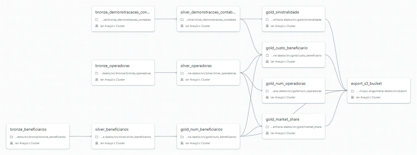
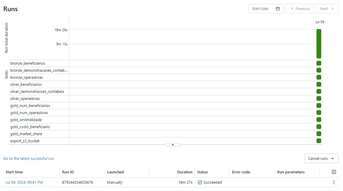
The pipeline ran for 18 minutes and 27 seconds, and all tasks completed successfully. For a big-data batch workload, that is not especially long, although the code could be made more efficient or run on larger clusters.

Data analysis

I built the analytics environment separately from Databricks, using Metabase on AWS and Docker. The gold-layer tables were loaded into a PostgreSQL database, where I could run queries, answer the questions defined at the start of the project, and create visualizations.

I could have answered the questions in Databricks, but chose to build a separate analytics environment with Metabase, an open-source BI and dashboard service. In Metabase, SQL queries can be saved as “Questions,” organized into collections, and used to build dashboards.

1. What is the current medical loss ratio in the health-insurance sector? Is it above or below its historical average?

The medical loss ratio is an important profitability indicator for insurance. In the medical and hospital-plan segment, it is the ratio of covered medical expenses (claims) to revenue earned from health plans.

A high ratio means a large share of revenue is being spent on claims. It may indicate that premiums need adjustment or services need to be reviewed to maintain the insurer's financial sustainability.

A very low ratio could point to an uncompetitive operation or underuse of health services. This also needs careful monitoring to maintain a fair balance between service delivery and financial viability.

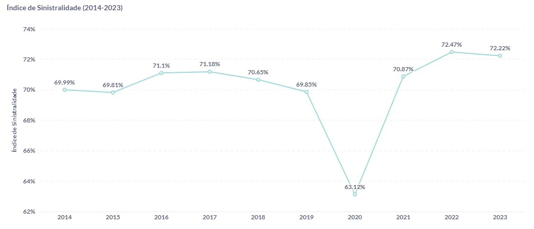
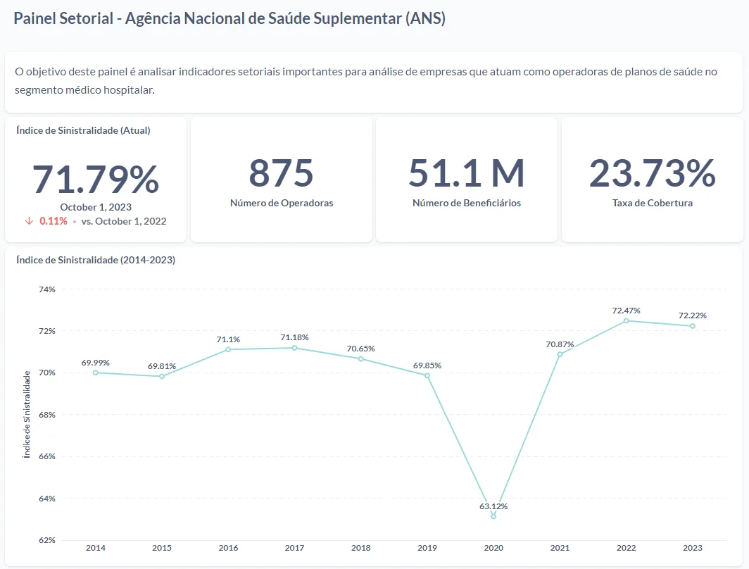
The current loss ratio is 71.79%, slightly above the historical average of recent years.

The chart's most striking feature is the unusually sharp drop in 2020, when the COVID-19 pandemic began and demand for medical care fell significantly. This may seem counterintuitive, but people postponed consultations, routine tests, and non-emergency procedures, lowering the loss ratio. After lockdowns, pent-up demand caused a sharp increase, leaving many companies in the sector under financial pressure.

2 and 3. Which insurer is most efficient in terms of cost per member?

Cost per member is an efficiency metric that estimates how much an insurer spends, on average, to provide healthcare services to each member over a year.

Insurers follow different business models and therefore have different cost structures. More vertically integrated companies—those that own hospitals, clinics, and laboratories—tend to have greater control over operations, costs, service quality, and intermediaries.

Market share, or a company's size relative to competitors, can also affect cost per member. Here, market share is measured by the number of members. Larger companies in this sector often benefit from economies of scale, optimizing resources and negotiating better prices for medicines and equipment.

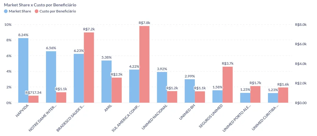
Hapvida, the sector's leader, recently acquired Notre Dame Intermédica and its hospital network, creating a group with almost 15% of the health-plan market, or about 7.65 million members.

Hapvida and Intermédica are vertically integrated: they sell health plans and own the hospitals that serve their members. This gives the company more control over margins and allows it to benefit from economies of scale.

Together, these factors help explain why the company has one of the lowest costs per member in the market—and the lowest among the ten largest insurers, at only R$717.54 per member per year.

At the other end of the spectrum is Bradesco Seguros, which has no owned hospital network and outsources the services provided through its plans. At the time of the analysis, Bradesco was the second-largest company if Hapvida and Intermédica are considered together, with an average annual cost of R$7,200 per member.

4. How many health-plan companies operate in Brazil?

At the time of this analysis, there were 850 active insurers in Brazil.

5. How many people have health-insurance coverage in Brazil? What is the coverage rate?

Brazil had around 51 million members of medical and hospital plans, with or without dental coverage. Compared with a population of about 215 million, that represents a coverage rate of approximately 23%.

In other words, fewer than one in four people in Brazil had a health plan.

6. Are individual or group plans more common?

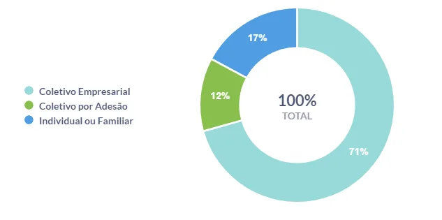
Of the more than 50 million members, only 17% had individual or family plans. The vast majority—83%—were covered by group plans, most of them employer-sponsored.

Metabase

In addition to Databricks, I built an analytics environment using Docker, PostgreSQL, and Metabase on an AWS EC2 instance.

I also wrote a Python script to perform a full load of the Parquet files stored in S3 into PostgreSQL tables. More information is available in the dedicated app/README.md, which explains how to configure the environment.

Besides using Metabase to query and visualize the data, I created a dashboard:

Conclusion

Overall, I found Databricks to be a very complete solution compared with the alternatives. Despite the additional cost, it offers many tools for data engineers, scientists, and analysts that can justify the expense through productivity gains.

Another important benefit was learning the platform and getting hands-on experience with features increasingly adopted by companies. It also made it possible to build solutions closer to those used in organizations. I recommend that anyone entering the field get some experience with Databricks.

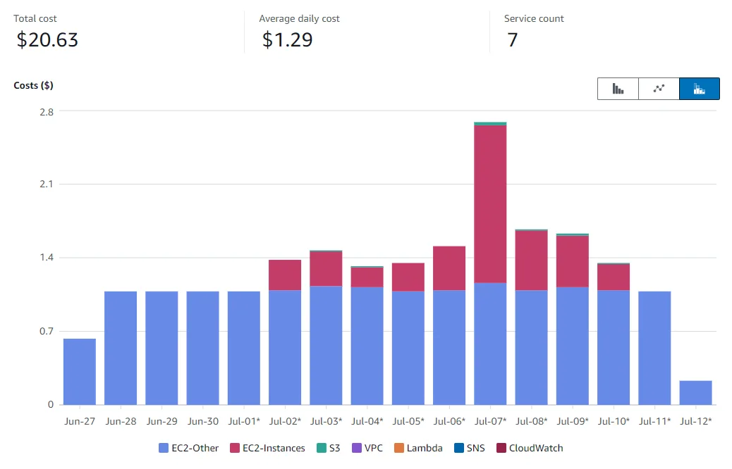
I planned to use the 14-day Databricks Premium free trial in full and set an AWS budget of about R$150 for the project.

I used a cluster with four cores and 16 GB of memory throughout the project. It proved sufficient for the workloads and offered a good balance between cost and performance.

From June 27 onward, the project cost a total of $20.63 (about R$120) across two main AWS services. The blue bars in the chart show a fixed cost essential to the Databricks workspace: the NAT Gateway, which provides network connectivity for the clusters. The red bars show the clusters used to run the project workloads.

Thanks for following along! :)